
[논문] YOLOv4: Optimal Speed and Accuracy of Object Detection
업데이트:
1. Introduction
- 가장 최신의 뉴럴 네트워크들은 실시간으로 작동하지 못하며 large mini-batch-size로 작동하기에는 많은 수의 gpu가 요구된다. 본 논문에서는 이런 점을 해결하고자, 기존의 한개의 GPU만을 이용하여 학습이 가능한 모델을 소개하고자 한다.
- Contribution
- 모델의 경량화(1080Ti 또는 2080Ti에서 돌아갈 수 있도록 하였다)
- SOTA Bag-of-Freebies와 Bag-of-Specials methods의 영향을 증명
- CBN, PAN, SAM 등을 포함한 기법을 활용하여 single GPU만을 이용한 효과적인 학습
- 1개의 GPU만을 이용하는 학습 환경에서 Bag-of-Freebies와 Bag-of-Specials methods를 통해 효율적이고 강력한 object detection을 제작하였다.
2. Related Works
2.1. Object detection models
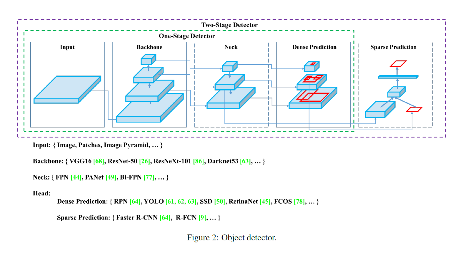
- Detector는 보통 두 파트로 구성되어 있다.
- Backbone: pre-trained on ImageNet, image를 feature map으로 변환
- Head: predict classes and bounding boxes
- Head는 Dense prediction/Sparse prediction으로 나뉜다. -> 1-stage/2-stage와 연관
- Sparse Prediction: 2-stage detector(ex.R-CNN, R-FCN), 클래스 예측과 box regression이 분리되어있음
- Dense Prediction: 1-stage detector(ex. YOLO, SSD), 클래스 예측과 box regression이 통합되어있음
- 자세한 설명은 link
- Neck은 backbone과 head를 연결하며 feature map refinement, reconfiguration
- FPN(Feature Pyramid Network), PAN(Path Aggregation Network), BiFPN, …
2.2. Bag of freebies(BoF)
- inference cost의 증가 없이 성능을 향상시키는 방법
- Data Augmentation: CutMix, MixUp과 같은 방식들을 이용
- BBox Regression의 loss함수를 이용하는것. (YOLOv3에서 이용함)
2.3. Bag of specials(BoS)
- inference cost가 상승하지만 성능향상이 되는 방법
- Enhance receptive field, feature integration, optimized activation function
3. Methodology
- For GPU: use small number of groups (1-8) in convolutional layers
- For VPU: use grouped convolution
3.1. Selection of Architecture
- 목표
- input network resolution, convolutional layer 개수, parameter 개수, layer output 개수 사이의 최적화된 균형 찾기
- 증가하는 receptive field에 추가적인 block과 다른 detector level을 위해 다른 backbone level로 부터 최고의 parameter aggregation을 선택하는 것
- classification을 잘하는 모델이 detector에는 꼭 최적화되어있다고 말할 수 는 없다
- detector는 아래 3가지를 요구한다
- Higher input network size: 여러개의 작은 object를 detect하기 위함
- More layers: 증가한 input network의 크기를 감당하기 위해 higher receptive field가 필요
- More parameters: 모델이 하나의 이미지에서 각각 다른 여러 물체를 감지하기 위해서 모델에 더 큰 용량이 필요로 된다
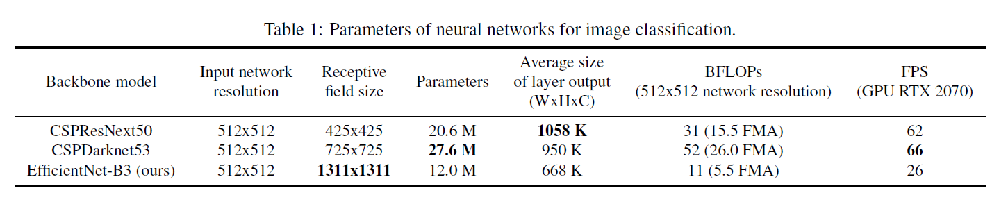
- Backbone model로는 큰 receptive field를 갖고 많은 수의 parameter를 갖는 모델이 선택되어야 한다고 한다 table 1을 참고하면 그 중 detector backbone으로는 CSPDarknet53이 가장 최적화 되어있는 모델이라 할 수 있다
- 각각 다른 사이즈를 갖는 receptive field의 영향은 아래와 같이 요약된다
- Up to the object size: 전체 object를 보는 것을 가능하게 한다
- Up to network size: object 주변의 context를 보는 것을 가능하게 한다
- Exceeding the network size: image poinㅅ와 final activattion 사이의 연관성의 수를 증가시킨다
- SPP block을 CSPDarknet53에 추가하여 receptive field를 매우 증가시키고, 가장 중요한 context feature를 분리시키고 network 작동시간에 거의 영향을 주지 않는다
- YOLOv3와는 다르게 parameter aggregation에는 FPN 대신에 PANet을 이용한다
- 이후에는 detector를 위해 BoF를 증가시킬 계획이다
- Cross-GPU Batch Normalization을 이용하지 않는다(초고사양의 GPU가 없어도 작동이 가능하도록 하고자 한다)
3.2. Selection of BoF and BoS
- Object detection training을 향상시키기 위해서 CNN은 아래의 기법들을 이용한다
- Activation: ReLU, leaky-ReLU, parametric-ReLU, ReLU6, SELU, Swish, or Mish
- Bounding box regression loss: MSE, IOU, GIoU, CIoU, DIoU
- Data Augmentation: CutOut, MixUp, CutMix
- Regularization method: DropOut, DropPath, Spatial DropOut or DropBlock
- Normalization of the network activations by their mean and variance: Batch Normalization, Cross-GPU Batch Normalization, Filter Response Normalization, Cross-Iteration Batch-Normalization
- Skip-connection: Residual connections, Weighted residual connections, Multi-input weighted residual connections, or Cross stage partial connections(CSP)
- Activation function을 학습하는데에 있어서 PReLU와 SELU는 학습시키는게 어렵고, ReLU6은 network의 quantization을 위해 디자인 되었으므로 후보군에서 이들은 삭제되었다
- Regularization의 방법으로 Drop Block을 소개한 논문에서는 다른 방법들과의 비교가 잘 이루어져 있었으므로 이를 선택하였다
- Normalization의 방법으로는 한 개의 GPU만을 이용하기 위해서, syncBN은 고려되지 않는다
3.3. Addtional improvements
- 한 개의 GPU만을 이용하여 학습하는 것을 가능하게 하기 위해 추가적인 설계를 하였다
- 새로운 방식의 data augmentation, Mosaic과 Self-Adversarial Training(SAT)을 추가
- 최적화된 optimal hyper-parameter를 적용하고자 한다
- 몇몇 현존하는 방법들을 모델에 적절하도록 조정한다
- Mosaic: 4개의 학습 이미지를 합치는 방식, large mini-batch의 크기를 줄이는 효과
- Self Adversarial Training: 새로운 방식의 data augmentation
- Crossed mini-Batch Normalization(CmBN)
- CBN modified version
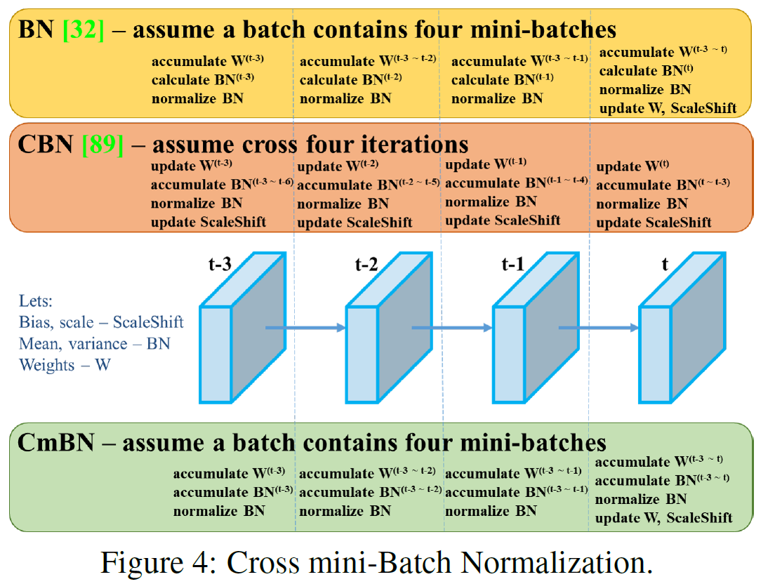
- CBN modified version
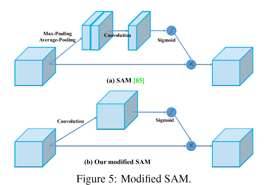
- SAM을 spatial-wise attention에서 point-wise attention으로 변경한다
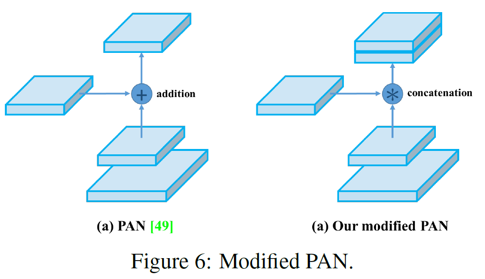
- PAN의 shorcut connection을 concatenation으로 대체한다
3.4. YOLOv4
사용된 Architecture
- Backbone: CSPDarknet53
- Neck: SPP(Spatial Pyramid Pooling), PAN(Path Aggregation Network)
- Head: YOLOv3
기법
- Backbone BoF: CutMix [link], Mosaic, DropBlock [link], Class label smoothing [link]
- Backbone BoS: Mish Activation [link], Cross-stage partial connections [arxiv], Multi input weighted residual connections(MiWRC)
- Detector BoF: CIoU-loss [arxiv], CmBN [arxiv]
- Detector BoS: SPP-block [arxiv]/[link], SAM-block [arxiv]/[link], PAN path-aggregation block [arxiv]/[link], DIoU-NMS
4. Experiments
Classifier에 대한 정확도는 ImageNet, Detector에 대한 정확도는 MS COCO 데이터 셋으로 측정한다.
4.1. Experimental setup
ImageNet image classification
- Training steps: 8,000,000
- Batch size, mini-batch-size: 128, 32
- Polynomial decay learning rate: 0.1, Warm-up steps: 1000
-
Momentum: 0.9, Weight decay: 0.005
- BoS experiment
- default hyper parameter
- compare LReLU, Swish, Mish activation function
- BoF experiment
- additional 50% training steps
- verify MixUp, CutMix, Mosaic, Bluring data augmentation, label smoothing regularization method
- GPU: 1080Ti or 2080 Ti
MS COCO object detection
- Training steps: 500,500
- Initial learning rate: 0.1 (strategy decay learning rate adopted, multiply with a factor 0.1 at the 400,000 steps and the 450,000)
- Batch size, mini-batch-size: 64, 8 or 4 (depend on GPU memory limitation)
- Momentum: 0.9, Weight decay: 0.0005
- Genetic algorithm used YOLOv3-SPP to train with GIoU loss and search 300 epochs
-
Learning rate: 0.00261, momentum: 0.949, IoU threshold: 0.213, Loss normalizer: 0.07
- BoS experiment
- Mish, SPP, SAM ,RFB, BiFPN and Gaussian YOLO
- BoF experiment
- grid sensitivity elimination
- mosaic data augmentation
- IoU threshold
- genetic algorithm
- class label smoothing
- cross mini-batch normalization
- self-adversarial training
- cosine annealing scheduler
- dynamic mini-batch size
- DropBlock
- Optimized Anchors
- different kind of IoU losses
- GPU: only one
4.2. Influence of different features on Classifier training
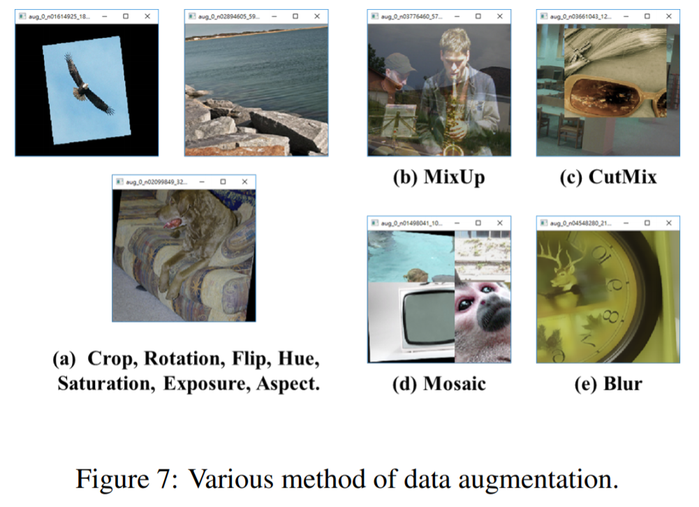
- 위의 이미지는 해당 기법들이 적용되었을 때의 예제 이미지이다
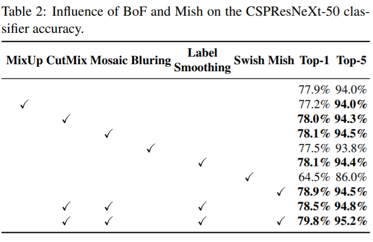
- 이 실험에서는 Table 2에 제시된 것 처럼 각 기법을 이용하였을 때 classifier의 정확도가 상승했는지를 확인하고자 한다
- 결과적으로 BoF backbone은 CutMix, Mosaic Augmentation, Class label smoothing을 포함한다
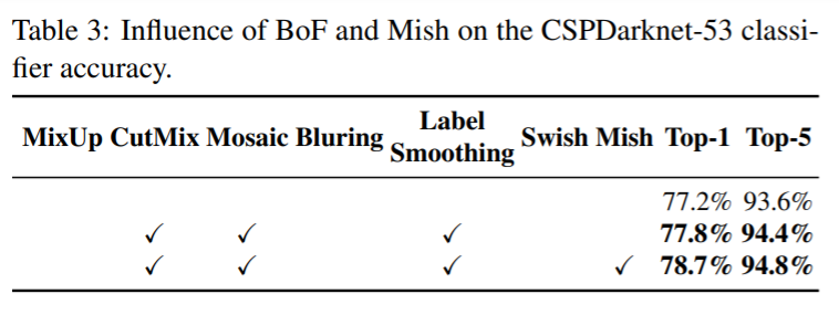
- 추가적으로 Mish activation을 보충적 옵션으로 사용하며 이에 대한 것은 table 2와 3에서 확인할 수 있다
- CutMix, Mosaic Augmentation, Class label smoothing과 Mish activation을 이용한 실험이 가장 결과가 좋음을 확인 (CSPResNeXt-50)
- 마찬가지로 CutMix, Mosaic Augmentation, Class label smoothing과 Mish activation을 이용한 실험이 가장 결과가 좋음을 확인 (CSPDarknet-53)
4.3. Influence of different features on Detector training
FPS에 영향을 미치지 않으면서 detector의 성능을 향상시키는 BoF의 영향에 대해서 알아본다
Influence of BoF
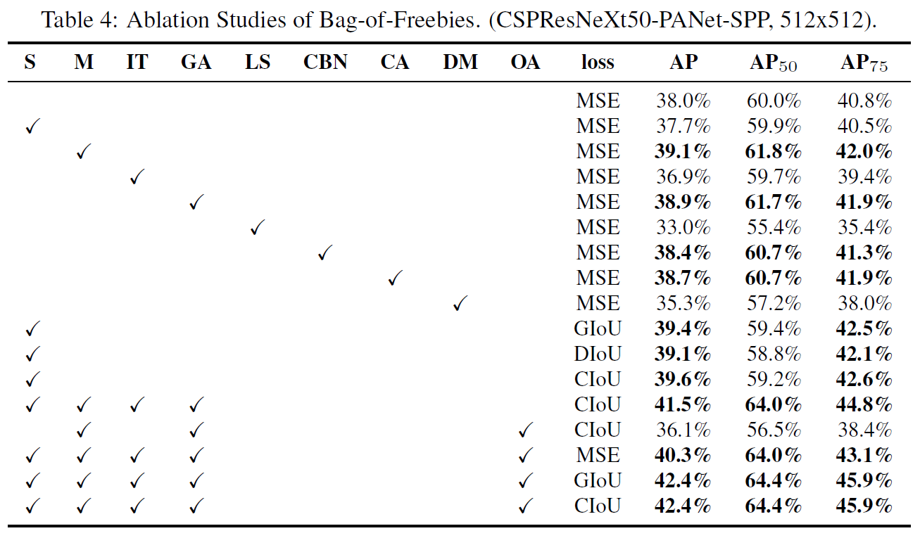
- S: grid sensitivity를 제거한다.
- M: Mosaic data augmentation - 훈련시 4장의 이미지를 한번에 사용한다
- IT: IoU threshold - single ground truth IoU에 여러 개의 anchor를 이용한다 (truth, anchor) > IoU_threshold
- GA: Genetic algorithms - network를 훈련시키는 동안의 첫 10%의 시간 동안 최적의 hyperparmeter를 위해서 genetic algorithm을 이용한다
- LS: class label smoothing - sigmoid activation을 위해서 class label smoothing을 사용
- CBN: CmBN - single batch에서 수집하는것 대신 전체 batch안에서 통계를 수집하기 위해서 Cross mini-batch normalization을 이용
- CA: Cosine Annealing scheduler - sinusoid(?) training시 learing rate를 변경한다
- DM: Dynamic mini-batch size - random training shape를 이용하여 small resolution training을 하는 동안 자동적으로 mini-batch 크기를 증가시킨다
- OA: Optimized Anchors - 512\(\times\)512 network resolution을 이용하여 학습하는데에 최적화된 앵커를 이용한다
- GIoU, CIoU, DIoU, MSE: bounded box regression을 위해서 다른 종류의 loss 알고리즘을 이용한다
Influence of BoS
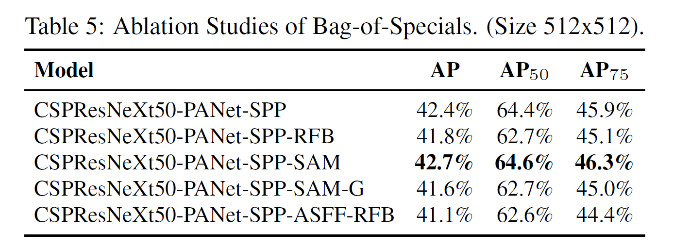
- SPP, PAN, SAM을 이용할 때 가장 좋은 성능을 보인다
4.4. Influence of different backbones and pretrained weightings on Detector training
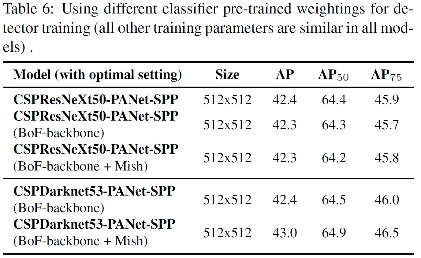
- classification에서 좋은 성능을 보인다 해서 detector에서 좋은 성능을 보이는 것은 아니다
- 첫째로, CSPResNeXt50이 CSPDarknet53보다 분류 정확도는 높지만 detection의 경우에는 CSPDarknet53의 성능이 더 좋다
- 둘째로, BoF와 Mish를 CSPResNeXt50에 사용하는 것은 정확도를 높이는데에 도움이 되지만 detector의 성능을 낮추는 것을 확인하였다. 하지만, CSPDarknet53에 BoF와 Mish를 사용하는 것은 분류와 감지 모두의 정확도를 상승시켰다
- 이는 Darknet53이 detector에 더 적합하다는 것을 보여준다
4.5. Influence of different mini-batch size on Detector training
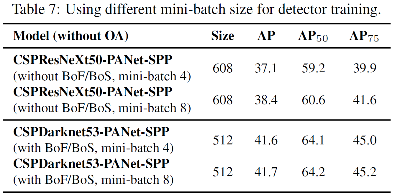
- Table 7의 결과를 통해서 BoF와 BoS를 거치고 난 뒤에는 mini-batch의 크기는 거의 영향이 없으며, 이는 더 이상 값비싼 GPU를 이용하여 학습할 필요가 없음을 보여준다
5. Results
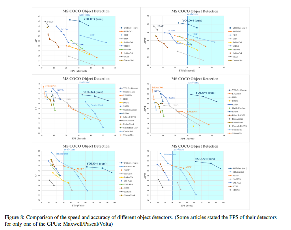
- Figure 8에서 다른 SOTA 모델들과 비교한 값을 확인할 수 있다
- 각 표는 왼쪽은 AP, 오른쪽은 AP50이며 각 GPU 모델별로 성능을 비교한 것의 그래프이다
- 그래프를 통해 YOLOv4가 속도 그리고 정확도 모두에서 다른 모델들과 비교했을 때 좋은 성능을 보임을 확인할 수 있었다.
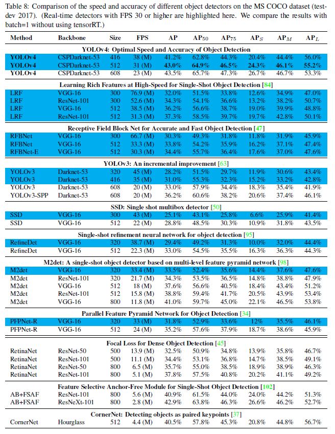
- Table 8은 각각 다른 architecture에 대해서 GPU의 영향을 보인다
- GTX Titan X 또는 Tesla M40를 이용할 때의 값
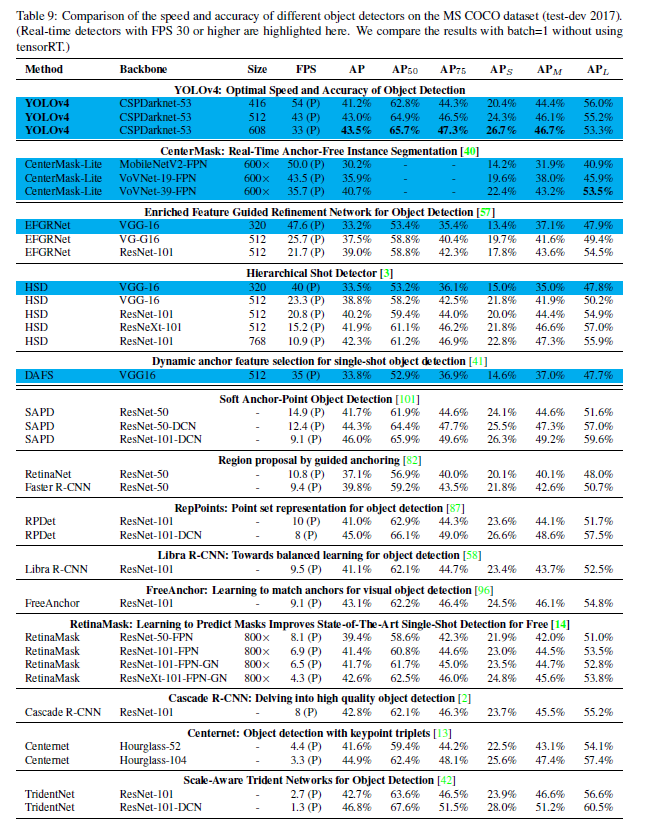
- Table 9은 각각 다른 architecture에 대해서 GPU의 영향을 보인다
- Titan X(Pascal), Titan Xp, GTX 1080 Ti, Tesla P100
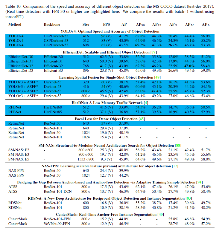
- Table 10은 각각 다른 architecture에 대해서 GPU의 영향을 보인다
- Volta GPU를 이용한 값이다
6. Conclusions
- 더 정확하고 더 빠른 모델을 제시하였다
- 8~16GB의 conventional한 GPU를 이용하여도 학습이 가능하다는 것을 보여주었다
- 다양한 feature의 성능을 검증하였고, classifier와 detector 모두에 도움이 되는 방식을 이용할 수 있었다
- 이러한 검증은 이후의 연구와 발전에 도움이 될 것이다
댓글남기기